Paper Machine Moisture Control

Setup

The systems are linearized around the operating point:

• valve opening: 80%
• steam pressure: 100 kPa
• moisture: 4.5%

The system’s linear model is given as:

Part I

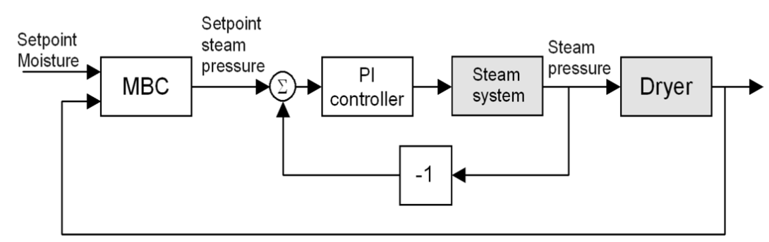
For part 1, we are tasked to design and simulate the PI controller for the inner loop of the casecade system. The paper by Slätteke on PI/PID tuning for IPZ processes suggests the following two implementations:

Where the IPZ process is generalized as:

I choose to implement option 1 as it is described to be better for rejecting disturbance. The system block model for the inner system looks like this:

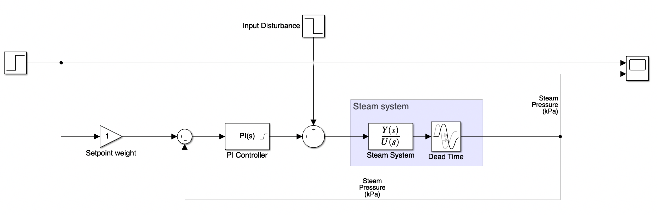
The PI controller is using the SimuLink built-in PID block with D component disabled, and with a saturation of [0, 100]. The calculated P and I gains from the Slätteke is as follows:

% Extract parameters for tuning from plant
L = steam_delay;
k_v = 0.006;
T_1 = 200;
T_2 = 80;

% Implementation 1 (disturbance rejection, Slätteke 2002)
k_c = 0.17 * T_2 / (T_1 * k_v * L);  % k_c = 11.3333
T_i = 3 * L * (31 * T_2 + 4 * L) / (7 * T_2 + 88 * L); % T_i = 11.5000

System Response

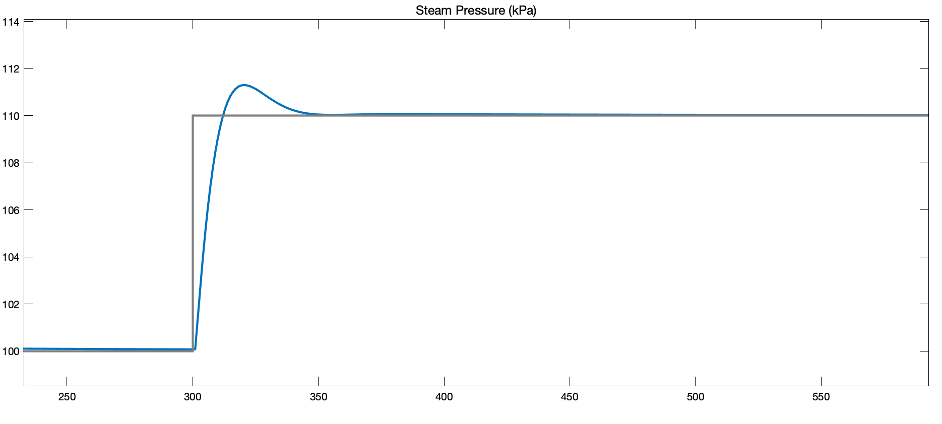
To test the response of the system, we set the initial condition of the steam system to have a pressure of 100 kPa. But because the system is linear, it is the Then we apply a step response of +10 kPa change to the setpoint. Here is the step response:

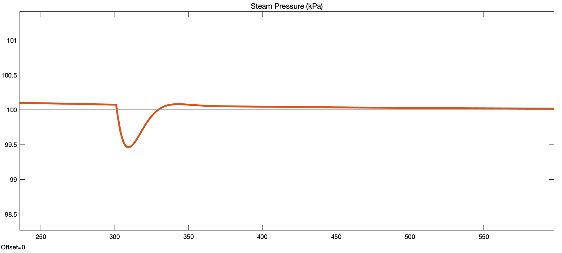
Next, we show that the system properly rejects a -10% valve openning input disturbance to the plant.

Part II

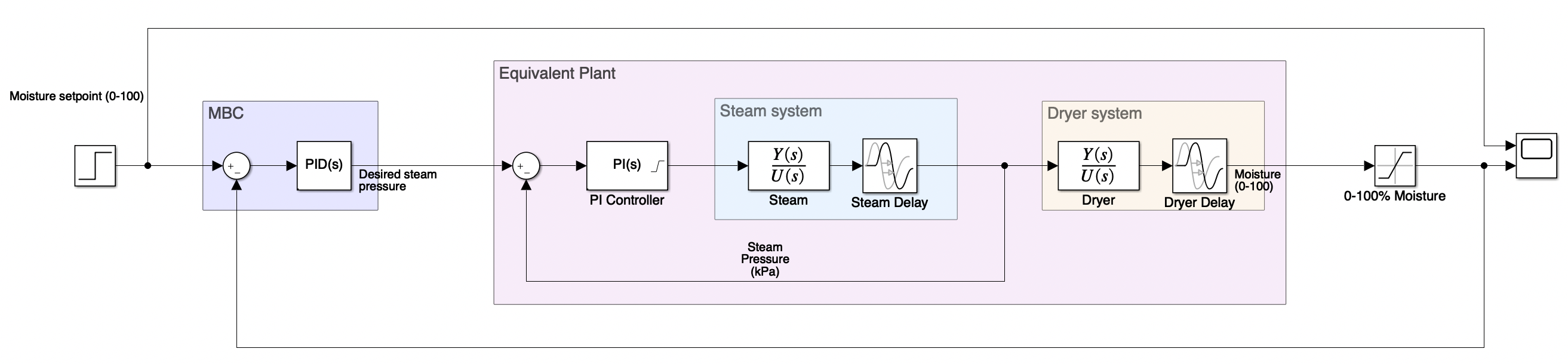
Now that we have the inner cascade system controlled to a reasonable degree, we can approxiamate it as part of our “outer plant” so that we can design the outer controller. As seen in the block diagarm below, let us denote $G_{eq}(s)$ as the plant transfer function that include the inner control loop as well as the dryer system.

The equivalent transfer function is given by:

To make the math a little easier, we neglect the dead-time for the inner system (remove the $e^{-s}$ term). The resulting equivalent transfer function is:

We will also define the equivalent plant transfer function without dead time as:

The root locus and bode plots for the above open-loop TF is as follows:

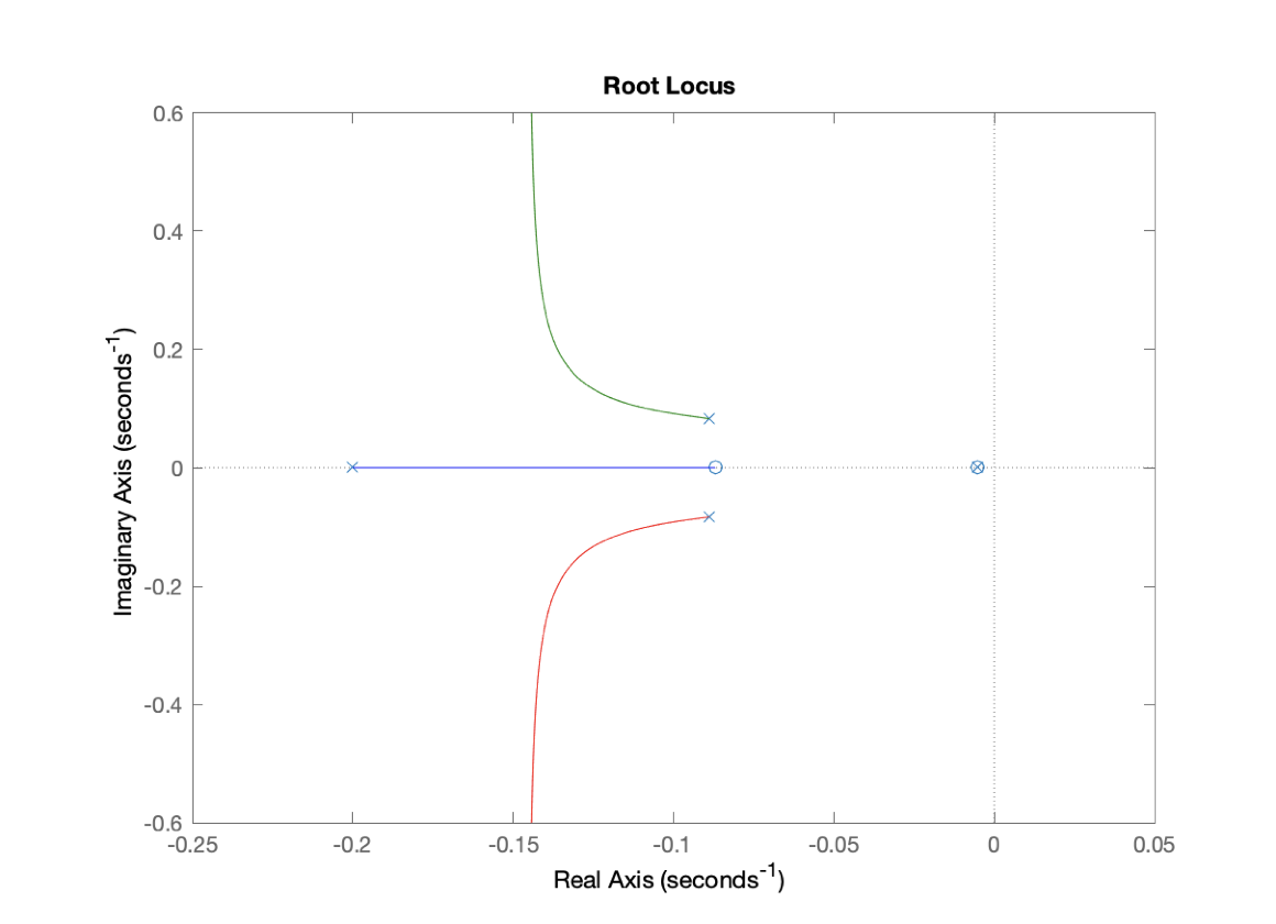
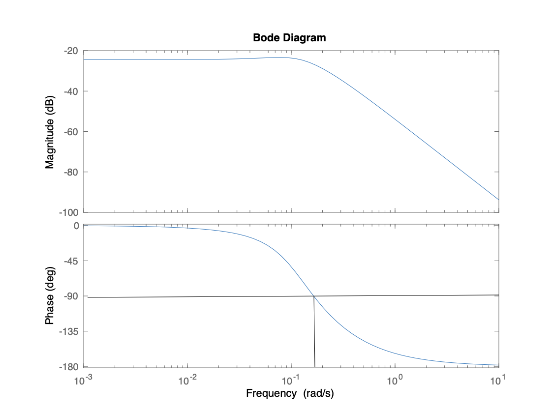
From the phase plot, we have an upper limit of our bandwidth of about 0.11 rad/s.

Using Q-Design as PID

From the above linearized equivalent transfer function of the plant (including the inner PI controller), we can devise a Q-design controller. $\bar G_{eq}$ is invertable with two zeros and four poles, so we need to add a filter $F_Q$ with two poles and unity gain:

Where we have chosen $\omega_n=0.1$ rad/s and damping $\zeta=0.6$ as it fits our model. Following the standard procedures for Q-design, we then have a controller

Using MATLAB to complete the numerical calculations for us, we finally get a PID controller for $C_Q$:

This corresponds to the form

Where $K_P=0.448$, $K_I=0.831$, $K_D=51.2$, and $\tau_f=11.5$.

Here is the block diagram implementation:

Note that we are expecting this design to do poorly because we have not yet accounted for the 40 second dead time. The actual response of the system is as follows:

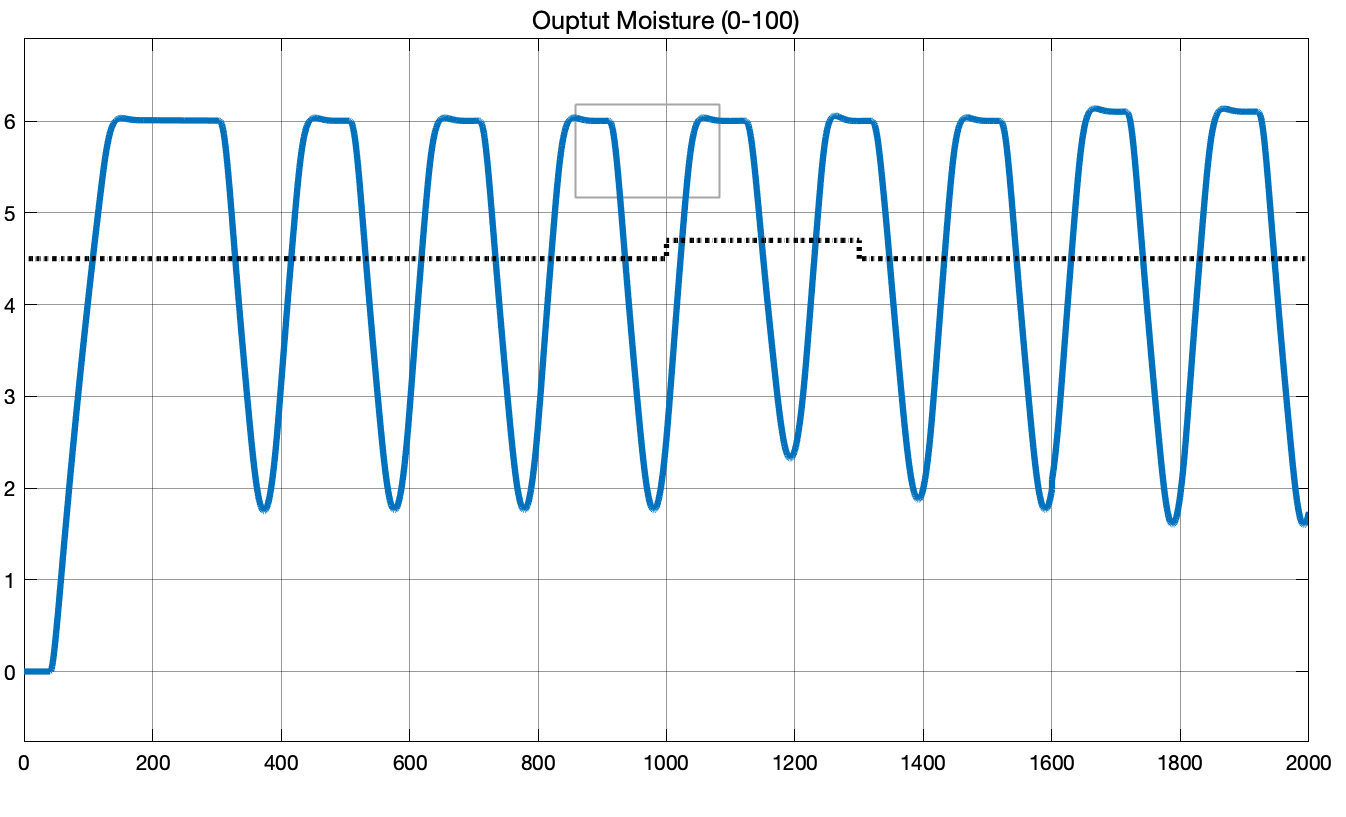
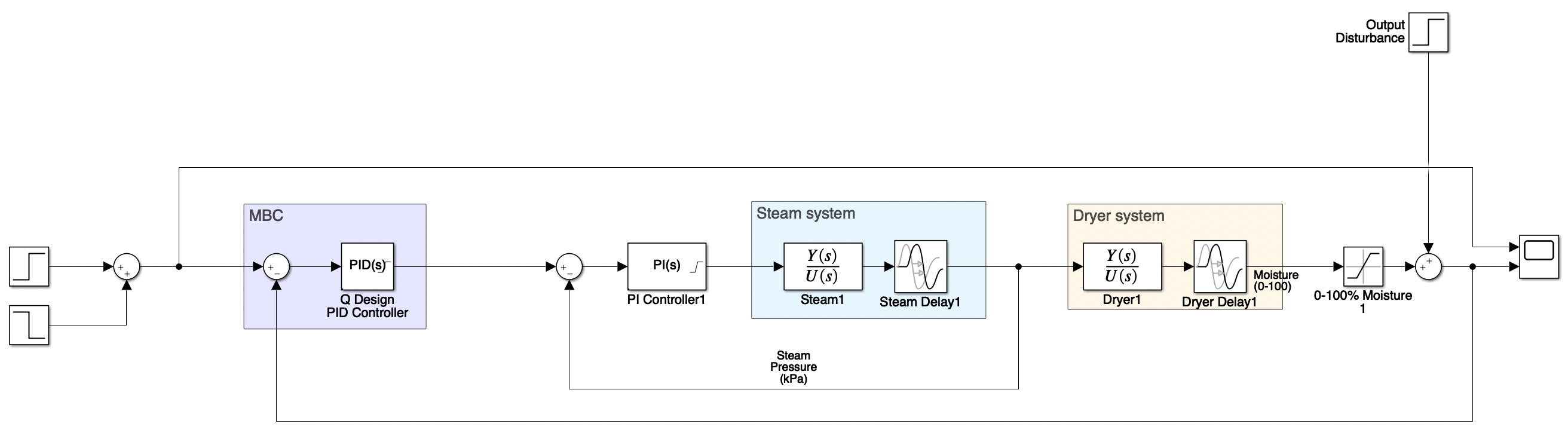
We see that the system is oscillating undesirably. Now let’s address the dead time by wrapping the PID controller inside a Smith Predictor as shown in the following block diagram:

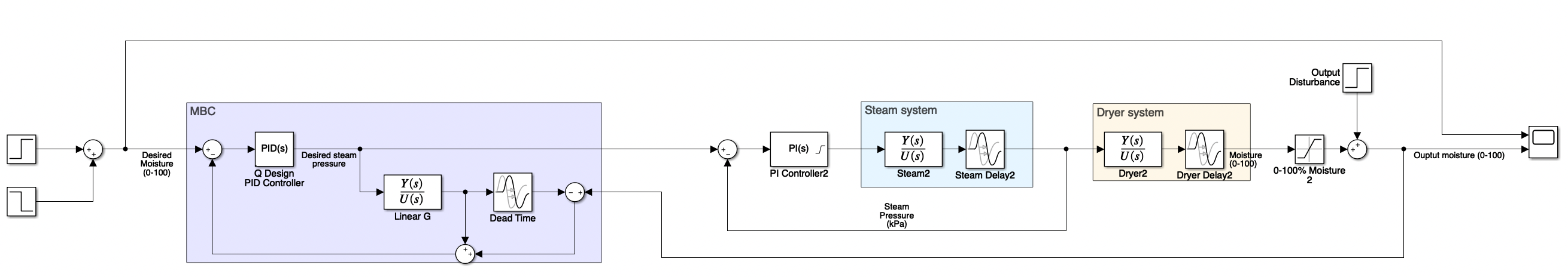
This block diagram encapsulates the entire system which is briefed in the project description. Now we are using a typical Smith Predictor to account for the 40 second dead time. The PID controller we obtained using Q-Design is now placed inside the MBC block with along with a linearized plant model Linear G feedforward block. The response is as follows:

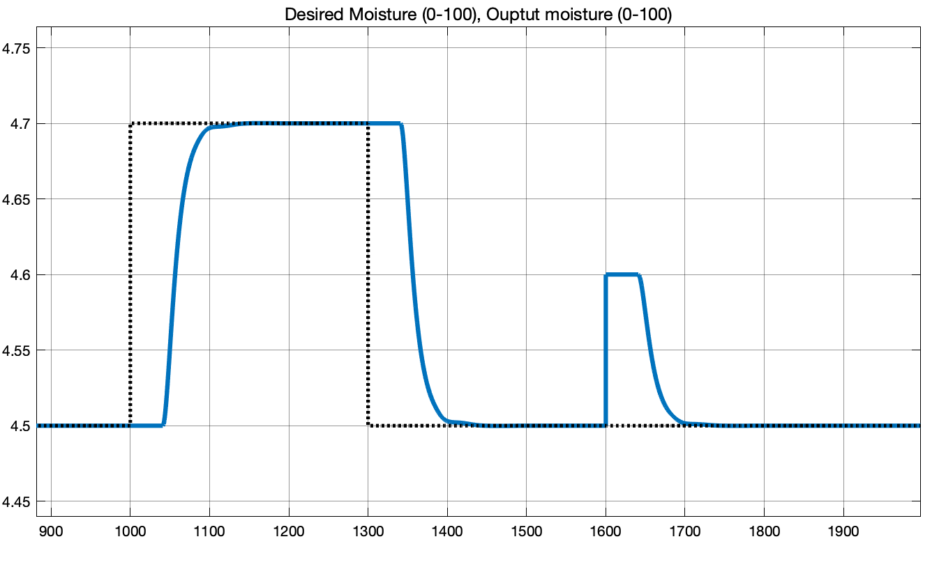
As we can observe that the same PID controller results in a much better behaved system thanks to the addition of the smith predictor. The desired setpoint rises from 4.5% to 4.7% moisture (0.2% increase) at time 1000. The entire system rises to desired setpoint within 100 seconds with 0% overshoot.

At time 1300, setpoint decrease back to 4.5% (0.2% decrease). We see that the system also responds adequately.

At tiem 1600, we apply an output disturbance of +0.1% moisture. Again, after a dead time of 40 seconds, the system quickly rejects output disturbance, and returns to the setpoint of 4.5% moisture.

MATLAB Code

Here are the MATLAB code used for setting up the variables in the workplace to be used in SimuLink.

% ELEC 441 Project
% Name: Muchen He
% Student ID: 44638154
%
% This file holds the model parmeters of the system in the project

% The following model parameters are derived with
% the system at a particular operating point:
% Valve opening: 80%
% Steam pressure: 100 kPa
% Moisture: 4.5%

clear;

% DSP tool box
s = tf('s');

% [PLANT] steam system
steam_num = [1.2, 0.006];
steam_den = [80, 1, 0];
steam_delay = 1;
steam_plant = tf(steam_num, steam_den, 'InputDelay', steam_delay);
steam_plant_lin = tf(steam_num, steam_den);

% [PLANT] dryer system
% dryer_num = [-0.06];
dryer_num = [0.06];
dryer_den = [5, 1];
dryer_delay = 40;
dryer_plant = tf(dryer_num, dryer_den, 'InputDelay', dryer_delay);
dryer_plant_lin = tf(dryer_num, dryer_den);

% Extract parameters for tuning from plant
L = steam_delay;
k_v = 0.006;
T_1 = 200;
T_2 = 80;

% Implementation 1 (disturbance rejection, Slätteke 2002)
k_c = 0.17 * T_2 / (T_1 * k_v * L);
T_i = 3 * L * (31 * T_2 + 4 * L) / (7 * T_2 + 88 * L);

% Implementation 2 (reference tracking, Slätteke 2002)
% k_c = 0.18 * T_2 / (T_1 * k_v * L);
% T_i = (L / 3) * (94 * T_2 + 13 * L) / (2 * T_2 + 29 * L);

% Compute PI controller parameters
K_P = k_c;
K_I = k_c / T_i;

% Ideal TF of the inner PI controller
C_inner = K_P + K_I / s;

% Equivalent cascade system
TF_inner = C_inner * steam_plant / ( 1 + C_inner * steam_plant );
TF_inner_lin = C_inner * steam_plant_lin / ( 1 + C_inner * steam_plant_lin );

% Equivalent plant (including dryer)
G_eq = minreal(TF_inner_lin * dryer_plant);

% Equivalent plant without dead time
G_eq_lin = minreal(TF_inner_lin * dryer_plant_lin);

% [Q-Design] Inverted non-dead-time model
G_eq_lin_inv = 1 / G_eq_lin;

% [Q-Design] F_Q filter
omega_n = 0.1;
damping = 0.6;
F_Q = omega_n ^ 2 / (s ^ 2 + 2 * omega_n * damping * s + omega_n ^ 2);

% [Q-Design] Controller
Q = F_Q * G_eq_lin_inv;
C_lin = minreal(Q / (1 - ( Q * G_eq_lin)));
C_lin_pid = pid(minreal(zpk(C_lin), 0.07));