Terrain Generator - Part 1: Theory

• What is a height map?
• Populating the height map
• Infinite Terrain
• Terrain Colours
• Next Steps

Let’s make a simple height-mapped based terrain generator. We will use Processing 3 for this project because it is easy to write code in 3D.

To represent the terrain, we will use a height map. To generate the height map, we use a noise function that takes in spacial coordinates and returns a seemingly “random” value.

What is a height map?

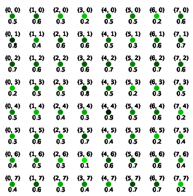
A height map is basically a 2D array where the x-y coordinates corresponds to the i and j indices of the 2D array, and the value of the element is the height.

The advantages of a height map is that it is easy to implement and fast to generate, it can create “macroscopic” terrain that is good enough for now. However, there are as few disadvantages: for one, we are limited to a single type of non-deformed topology (imagine a sheet of paper that can only be crumpled but cannot be rolled, torn, or folded). When there is large amplitutude, the terrain could also look very spiky.

Certain terrain generators use a voxel-based engine, which instead of using a 2D array, it uses a 3D array to keep track of every spatial unit, allowing for more complex structures like caves and overhangs.

Populating the height map

As mentioned before, we need a noise function to populate the elements in the height map 2D array. A noise function typcially takes in some spacial coordinates (x, y, and/or z) and outputs a single value typically clampped between 0.0 and 1.0. Since we’re populating a 2D array here, we will use a 2D noise function, something like: float noise(float x, float y).

There are also many types of noise functions. The most commonly used are Perlin noise and Simplex noise. Perlin noise is built into Processing 3 so we will use that, eventhough Simplex noise usually looks more organic.

Note that we must multilpy x and y by some scaling factor s to make the output look smooth. Let’s make s = 0.001 to start. This is essentially our spatial “frequency”.

To make the terrain look realistic, we add the harmonics of the noise function together. A reasonable amount is at least 3 octaves and for each octave. For each octave, we double the frequency and decrease the amplitude by half (suggested reading: ¹). So for each element in the array, it can be expressed using the math equation:

\[H_{x,y}=N(sx, sy)+\frac{1}{2}N(2sx, 2sy)+\frac{1}{4}N(4sx,4sy)+\dots\\ =\sum_{n=1}^{k}\frac{1}{2^{n-1}}\cdot N(2^{n-1} sx,2^{n-1} sy)\]

Infinite Terrain

The noise function can handle a range of inputs from -∞ to ∞. So we could create infinite terrain. But obviously we cannot have a infinitely sized 2D array, what do we do?

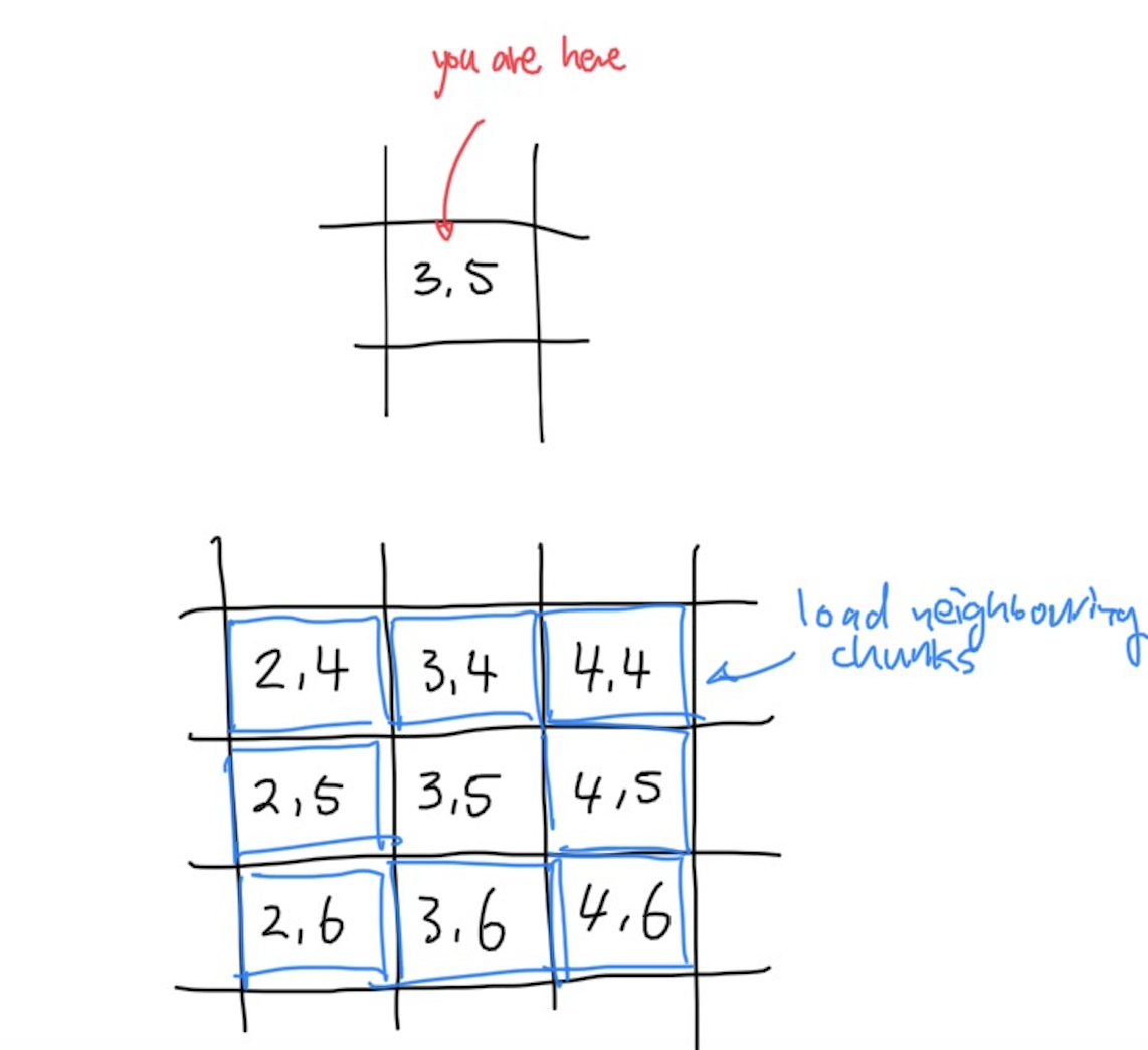
The answer is chunks, like Minecraft. Basically, we break up the terrain into many smaller grids of 2D arrays, and only load the ones we can see.

It is not a big change as we just need to keep track of a list of 2D arrays, our current position, and some metadata for each chunk. Suppose our current coordinate is centered around chunk (3,5), then we can load the chunk we’re currently in (3,5) as well as neighbouring chunks (2, 4), (2, 5), (2, 6), (3, 4), (3, 6), (4, 4), (4, 5), (4, 6). Of course, we can always increase the “viewing radius” to load and display more neighbours.

When we move our camera around, we can refresh the terrain by unloading the chunks that are too far away, and at the same time load new chunks that are now close enough for us to see.

Terrain Colours

For the sake of simplicity, we can assign a gradient of color for each of the verticies in the 2D array based on altitude. We will use the following simple linear gradient:

<div style=“height=30px; width=100%; background: linear-gradient(90deg, rgba(70,53,32,1) 8%, rgba(242,236,193,1) 18%, rgba(57,75,52,1) 30%, rgba(133,175,136,1) 84%, rgba(255,255,255,1) 93%);”></div> We can plot the points on a graph and obtain a mathematic function for each of the RGB curves (which makes it easier to implement in Processing 3).

\[R(x)=e^{-0.01\left(x-18\right)^{2}}\cdot240+e^{0.07\left(x-13\right)}\\ G(x)=e^{-0.012\left(x-19\right)^{2}}\cdot225+e^{0.04\left(x+45\right)}\\ B(x)=e^{-0.013\left(x-19\right)^{2}}\cdot190+e^{0.07\left(x-14\right)}\]

Plotted:

Next Steps

In part 2, we will code all of the above up in Processing 3 so stay tuned.