Last updated 2018-06-20 by Muchen He (44638154)
Assignment 2Problem 1DescriptionAnalysisEndowment FundConclusionProblem 2DescriptionAnalysisEconomic CriteriaStrategiesNumber CrunchingStrategy 1Strategy 2Strategy 3Strategy 4NPV AnalysisEACF AnalysisConclusionExtra FactorsProblem 3AnalysisDo NothingJob 1Job 2Incremental AnalysisLine of Credit
Assignment 2
Problem 1
Description
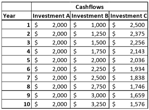
At an 8% interest rate, if you were to invest $10,000 into one of the following investments, which one should you choose? Which factors (e.g. Single Payment Compound Amount Factor) would you use to evaluate each investment?
If you instead decided to donate the $10,000 to an endowment fund for a charity you favour, how much annual revenue would the charity receive from your gift, assuming the same 8% interest? What would the Future Value of the endowment be?
Analysis
Investment A is a uniforms series because of its uniform cashflows. Investment B is arithmetic series as the cash flow increases linearly at $250 each period. Investment C is a geometric series except the growth is actually negative. Investment C's growth is -5%.
Investment A
For investment A, we look at its uniform series present worth factor. We use the formula with and .
Investment B
For investment B, we will utilize arithmetic gradient uniform series factor to turn the periodically increasing cashflow into an equivalent cashflow. Let be the uniform cashflow (since the first cashflow is $1000). Let . Then we use the formula to get equivalent annuity:
Then apply the same method used for investment A using the equivalent arithmetic gradient uniform series factor to find the present worth factor. Except we include the original uniform cash flow as well as the equivalent cash flow of the arithmetic series:
Investment C
This is a geometric series with growth rate . Because , we apply the present worth factor formula:
Endowment Fund
Note: endowment fund is donating $10000 and only getting the gain from the interest rate.
If we instead decide to donate $10,000 to an endowment fund, then the annual revenue is 8% of $10000, which is $800, because the following year will be at $10,000 again.
The future value is calculated using compound amount factor:
Conclusion
Given option A, B, C, one should choose investment C because it has the highest present value. If we donated the $10,000 to the endowment fund, we would get an annual revenue of $800 with future value of $11,589.
Problem 2
Problem 2 Excel sheet and scrap work available here.
Description
SAN Swiss Arms is a Switzerland based manufacturing company that makes firearms. Swiss Arms is considering manufacturing a rifle for sale in Canada. Canada is a small market for their product, but they have an existing design they could use. However, it would need to be modified to meet Canadian firearms legislation. The engineering and testing work for the design changes are estimated to be 875,000€.
Swiss Arms estimates they will sell 1,000 rifles in the first year of production, increasing linearly to 1,450 rifles in the 10th year. The rifles sell for 1,425€ each.
Rifle production can be done on an existing production line, except the new design requires one process to be modified. This can be done manually, which would incur no capital costs and give a cost per rifle of 1,150€. Alternatively, Swiss Arms can purchase a new tool for the process which would cost 240,000€. It will give a cost per rife of 1,060€, but the tool is only good for four years and has no salvage value.
Evaluate the alternatives using both NPV and EACF. If Swiss Arms considers 13.5% to be its interest rate, should they proceed with the project? If so, which alternative should they choose?
Bonus Questions: SAN Swiss Arms rifle have been involved in some legal/political controversy in Canada over the last few years. What kind of things can Swiss Arms do in this analysis to account for this risk?
Analysis
Note: NPV stands for net present value. EACF stands for equivalent annuity cashflow.
First, our gathered known variables are as follows:
| Initial design cost (one time) | 💶875,000 |
| Revenue per rifle | 💶1,425 |
| Cost (manual) per rifle | 💶1,150 |
| Cost (with tools) per rifle | 💶1,060 |
| Tools cost (one time) | 💶240,000 |
| Interest rate | 📈13.5% |
| Initial estimated sale (year 1) | 🔫1000 |
| Final estimated sale (year 10) | 🔫1450 |
Let's assume that the growth of sales per unit increases linearly from 1000 to 1450 per year. Since the variable cost and revenue is uniform over time, this forms a linearly increasing cashflow. Thus, we will use the arithmetic series to model.
Economic Criteria
We notice that our input is not fixed as we can have varying costs. But our output is somewhat fixed, because we need to meet the requirements of the estimated sale volume.
Thus, in NPV analysis, our criteria is to minimize the present worth cost and maximize the net present value.
In EACF analysis we want to minimize the equivalent uniform annual cost (EUAC).
Strategies
The tools last 4 years but our analysis period is 10 years. We assume that the tools are repeatable purchases. There are a number of permutations on which when the tools can be bought. To keep the analysis simpler, let's assume that we can purchase the tools not once, once, twice, or three times; all consecutively after the last tool set fails starting at the beginning of year 1.
This leaves us with 4 main alternatives:
- Don't buy any tools
- Buy tools at the beginning of year 1 (end of year 0)
- Buy tools at the beginning of year 1 and 5
- Buy tools at the beginning of year 1, 5, and 9
Number Crunching
Strategy 1
For strategy 1, we compute the cost and revenue for each year and convert it to present worth using single payment present worth factor on each year, which is given as .
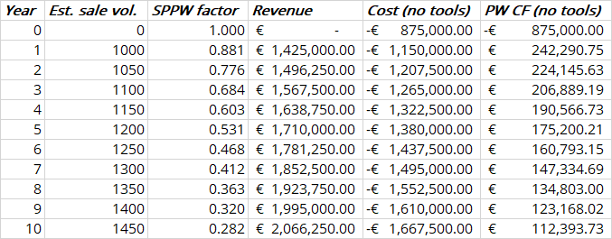
The sum of all the present worth cash flows for each year gives us the NPW: .
Strategy 2
Similar computation is applied for strategy 2. Note that we have an additional tool cost of $240k in year 0 (beginning of year 1).
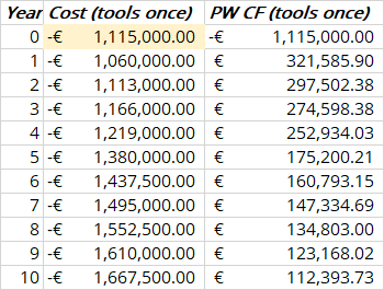
The NPW for this is .
Strategy 3
Same as strategy 2, except there is an extra tool cost at the end of year 4 (beginning of year 5) as well.
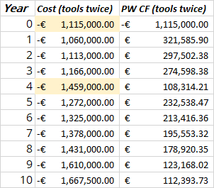
The NPW for this .
Strategy 4
We repurchase the tools every time for the entire analysis period. Note that we at the end of year 10, there still exists 2 years worth of useful life left, which is not as optimal.
The unused useful life is reflected in the NPW as it is which is less than strategy 3.
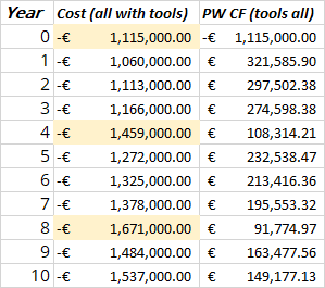
NPV Analysis
From the previous section we found the net present worth of each year. So the total net present value (NPV) would be the sum of all years. The table below shows the NPW for each strategy alternative:
| Strategy 1 | Strategy 2 | Strategy 3 | Strategy 4 | |
|---|---|---|---|---|
| NPV | € 842,585.11 | € 885,313.49 | € 942,991.12 | € 932,938.68 |
| PW Costs | € 8,057,628.63 | € 8,014,900.24 | € 7,957,222.61 | € 7,967,275.05 |
Out of all these options, strategy 3 is the best as it has the highest net present value, or the lowest present worth costs. This satisfies our economic criteria and thus should be our preferred choice.
EACF Analysis
From NPV analysis we have the net present value and present worth costs. We can obtain both the equivalent annual cashflow (EACF) and equivalent uniform annual cost (EUAC) using the capital recovery factor.
| Strategy 1 | Strategy 2 | Strategy 3 | Strategy 4 | |
|---|---|---|---|---|
| EACF | € 158,395.03 | € 166,427.41 | € 177,270.05 | € 175,380.32 |
| EUAC | € 1,514,729.26 | € 1,506,696.87 | € 1,495,854.23 | € 1,497,743.96 |
The EACF in this case is synonymous for equivalent uniform annual worth (EUAW). Given the economic criterion we want the lowest EUAC and highest EACF. Therefore our preferred choice is strategy 3 again.
Conclusion
From both NPV and EACF analysis, we see that strategy 3 is the most optimal. Where we purchase tools from the very beginning and replacing it once (tool is purchased twice in 10 years).
Extra Factors
There exists social externalities with this project that might ultimately affect the economic outcome. For example there might be social incentives to increase gun control or reduce gun license sales, which might hurt sale volume.
Some more factors that would need consideration in real life:
- Tariffs on contraband goods
- Lobbying / political influence such to maintain reputation
Problem 3
Problem 3 Excel sheet and scrap work available here.
Analysis
Do Nothing
This will give us an rate of return of 0%, which is strictly lower than the MARR of 19%. Therefore this approach will not be considered.
Job 1
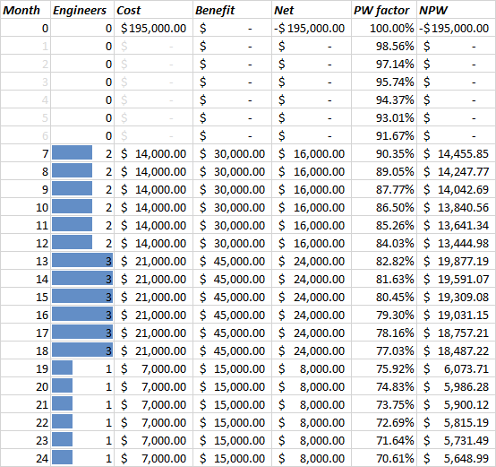
The proposal is submitted at the beginning of year 1 (or end of year 0) for $195k. Given the scenario, the project actually starts on month 7 with 2 engineers. This means that the analysis period for job 1 is actually 24 months.
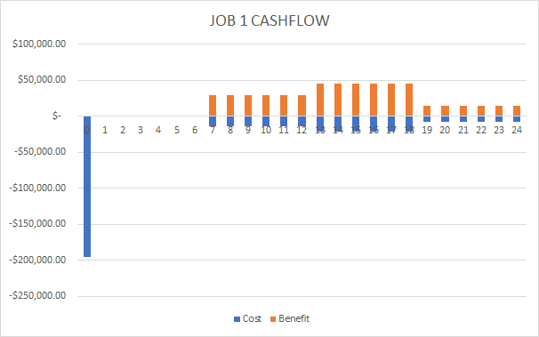
We compute the yearly costs and benefits given that the net income for each engineer is $8000 each. Below is the table of calculations and the cashflow diagram.
Using the definition for internal rate of return calculation, where present worth costs equal to present worth benefits (check the excel sheet for more details in calculation):
We isolate and solve for we get our equivalent monthly nominal interest rate. The nominal annual interest rate is then . Then formula we obtain the effective interest rate, where is 12 months in a year.
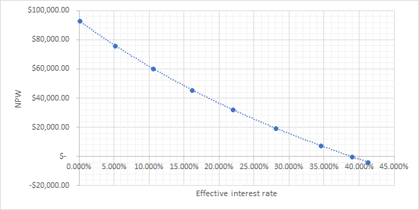
Finally, we get IRR of . This is more than the MARR of 19% which indicate that this could a viable solution. Furthermore, we can plot the NPV vs. effective interest rate graph:
Job 2
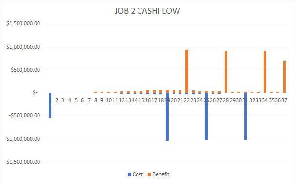
Similarly with job 1, we compute the annual cashflow with the bidding price of $535k. However, there are additional costs for construction:
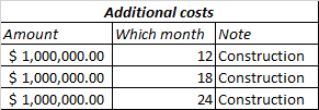
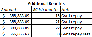
Along with, the government also reimburses the construction costs with 10% profit margin. This means that for $1M we spend for construction, the government will pay .
Because the government will hold on to 20%, they will only pay and the rest at the end:
For more details, consult the spreadsheet. The final cashflow diagram resembles as follows:
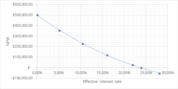
The exact same method for computing IRR is applied here and we get IRR of which is lower than that of job 1, but still greater than the MARR.
The NPV vs. effective interest rate graph is as follows:
Incremental Analysis
To compare the two alternatives, I assume that these projects can be purchased repeatedly. But each time purchased, a new proposal (along with the 6 month period) is required.
This enables a relatively easier analysis period, which is the LCM of 24 months and 36 months which is 72 months. Since the initial cost for job 2 is greater, we will take the difference of (cost of job 2 minus cost of job 1).
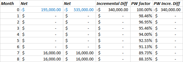
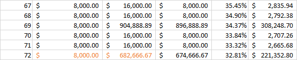
We find the present worth of the incremental difference as a function of and equate it to 0. This allows us to isolate for and find the monthly nominal interest of 1.56%.
Using identical computation as before, we find the effective annual interest, AKA IRR of . Sinc e the IRR is greater than the MARR. Our economic criterion states that we should go with the higher costing alternative, which is job 2.
Line of Credit
In this situation, we will employ the modified internal rate of interest (MIRR) technique. Since we have chosen job 2, we will use the cash flow presented from previous section.
- We separate the cashflow that is negative or positive based on net expense or income
- The expense is under influence of loan interest (0.53% monthly). We find the present value of $3.107M.
- The income is under influence of investment interest (0.81% monthly). We find the future value of $4.211M.
- The MIRR is adjusted such that PW = FW. The formula is:
Finally, MIRR is solved to be .